
Excel SUMIFS Counts the Wrong Product: Escape Literal * and ?
Use a visible literal-criterion helper and a five-row reconciliation to stop product-code wildcards from inflating totals.
Published November 15, 2026

If Excel SUMIFS returns too much for a product code containing * or ?, check whether the formula is treating that character as a wildcard. An asterisk matches a sequence of characters; a question mark matches one character. To total the literal product code AB*12, use AB~*12 as the criterion. Keep the actual product code unchanged in the source data.
For a report where the user selects a literal code in E2, use three short helper formulas: F2 escapes existing tildes, G2 escapes asterisks, and H2 escapes question marks. Use H2 as the final SUMIFS criterion. The formulas below keep each change visible and preserve the literal meaning of the original tildes. This is a repair for a defined identifier rule, not permission to change every report that intentionally uses pattern matching.
Decide whether the report means one code or a family
This guide is for a sales or finance analyst who totals transaction amounts by an exact product identifier. It fits an export where punctuation belongs to the code, such as a supplier's AB*12. It does not fit a report deliberately asking for all products beginning with AB, or a code system where upper- and lowercase letters identify different products without a separately designed case-sensitive comparison.
Microsoft's SUMIFS documentation, checked November 15, 2026, describes the wildcard behavior and the tilde escape. It also requires the criteria and sum ranges to have matching dimensions. The documentation establishes the formula mechanics. Whether AB*12 means one literal product or a product family is a business rule that the catalog owner must supply.
Write the rule above the selector: “Product code: exact literal identifier” or “Product pattern: * and ? are supported wildcards.” Do not leave the meaning implicit. The same entry can produce a plausible total under both interpretations, so a correct-looking number does not reveal which question the formula answered.
If both modes are needed, provide two clearly labeled reports or a visibly labeled mode selector with separate acceptance tests. Avoid having an analyst manually add tildes to some source codes. The source should continue to represent the catalog; the formula's helper represents the comparison rule.
Establish a small control sample
Work in a copy of the workbook and preserve the export. Name the source owner who can confirm the code system and the report owner who approves the total. Keep a dated source row count and grand total. The formula repair should change which rows belong to the selected product, not change transaction amounts or delete other products.
Use three columns for the first test: A contains Code, B contains Status and C contains Amount. Rows 2 through 6 will contain the constructed example below. Put the selected literal code in E2 and the three helper stages in F2, G2 and H2. Keeping the helpers visible makes review easier than burying multiple substitutions inside a long final formula.
This workflow uses functions documented for current supported Excel versions and needs no separate AI subscription or add-on. Its cost is analyst and catalog-owner time. Start with a small source sample before changing a shared management report. If the workbook drives commissions or purchasing, keep the original report available until the repaired logic is signed off.
Also confirm what Amount represents: net revenue, gross revenue, units or another measure. A correct character comparison cannot fix a report that mixes tax-inclusive and tax-exclusive amounts. Retain the existing approved financial definition while isolating the selection defect, then handle any separate measurement issue explicitly.
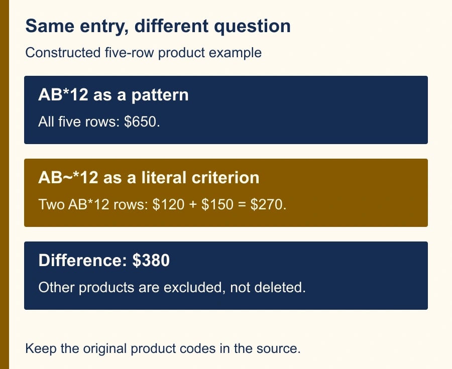
Worked example: $650 is a valid pattern total and a wrong product total
Create this constructed sample: row 2 is AB*12, Posted, 120; row 3 is ABX12, Posted, 200; row 4 is AB12, Posted, 80; row 5 is AB*12, Posted, 150; row 6 is AB?12, Posted, 100. These are illustrative transactions, not reported customer data. The grand total is $650.
Enter AB*12 in E2. The formula =SUMIFS(C2:C6, A2:A6, E2, B2:B6, "Posted") matches all five rows because the asterisk in the criterion can stand for any sequence, including no intervening character. It therefore returns $650. That is the total for the pattern beginning AB and ending 12, but it is not the total for the literal AB*12 product.
For the literal code, =SUMIFS(C2:C6, A2:A6, "AB~*12", B2:B6, "Posted") selects rows 2 and 5. The expected amount is $270: $120 plus $150. The difference is $380, representing the three other codes. Nothing is wrong with those three transactions; they simply do not belong in this product's subtotal.
Now select AB?12. Without escaping, the question mark matches one character between AB and 12. It matches rows 2, 3, 5 and 6, totaling $570, but excludes AB12 because that code has no intervening character. The literal criterion AB~?12 selects only row 6, for $100. Testing both symbols helps prove you have repaired the rule rather than memorized one special case.
Finally, select AB12. It has neither wildcard and should return $80 in this sample. An ordinary code is the control case: if it changes unexpectedly, inspect your ranges, status criterion or helper formula. The complete sample remains $650 whichever product you select; changing the selection does not change the underlying ledger.
Build a reusable criterion helper
Use three neighboring helper cells so the report owner can inspect the transformation:
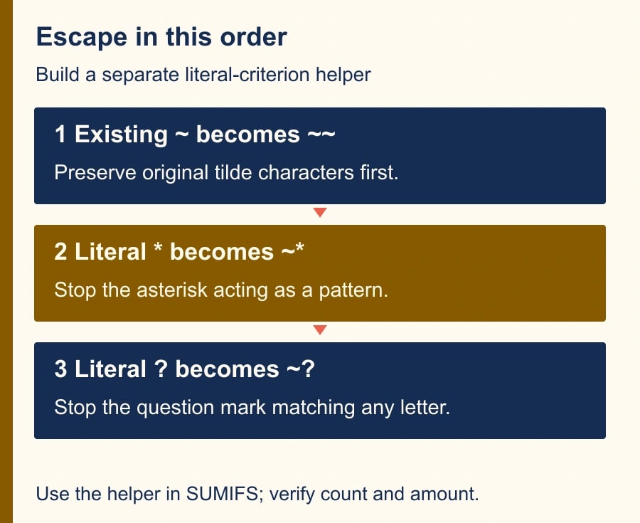
- In F2, enter =SUBSTITUTE(E2, "~", "~~") to escape the original tildes.
- In G2, enter =SUBSTITUTE(F2, "*", "~*") to escape literal asterisks.
- In H2, enter =SUBSTITUTE(G2, "?", "~?") to escape literal question marks.
H2 contains the final comparison text. Do not write it back into the catalog. For an ordinary code, all three helpers should retain the original value; for AB*12, the asterisk gains its tilde in G2 and H2 retains that result.
Microsoft documents SUBSTITUTE as replacing specified text, with all occurrences changed when no instance number is supplied. In this use, every occurrence needs escaping. Escaping only the first asterisk would leave another asterisk in a longer code active as a pattern instruction.
Order matters. If you add escape tildes first and then double all tildes, you also alter the escapes you just inserted. That can change the criterion's meaning again. The three-stage sequence above handles original tildes before introducing new escape characters. Keep a literal tilde example in the test pack even if the first failing product contains only an asterisk.
Use =SUMIFS(C2:C6, A2:A6, H2, B2:B6, "Posted") for the sample. The Amount range comes first in SUMIFS. Ensure every range starts and ends on the same data rows. In a production Excel table, use the corresponding table columns consistently so the source can grow without one range stopping earlier than another.
The examples use English function names and comma separators. Adapt separators to the workbook's locale if needed. Retain the ordinary straight quotation marks around text values. A formula pasted as plain text or with typographic quotation marks needs correction before its result can be judged.
Verify the selected rows as well as the sum
Add =COUNTIFS(A2:A6, H2, B2:B6, "Posted") beside the total. Microsoft's COUNTIFS documentation describes the same wildcard escape convention. In the sample, literal AB*12 should count two rows and total $270; literal AB?12 should count one and total $100. A count is a second diagnostic, not proof that the amounts themselves are correct.
For a hand check, compare each source Code with the selected code using a separate row-level equality check and inspect the included rows. Confirm that their status is Posted and add their amounts independently. Do not verify the repaired SUMIFS solely with a copied SUMIFS formula that contains the same mistake.
If the row count is correct but the amount is wrong, inspect number-versus-text amounts, signs, currency units and the amount range. If the count is wrong, inspect the criterion, the raw code characters and the status values. This split keeps the investigation focused. It prevents a punctuation fix from becoming an unreviewed rewrite of the whole workbook.
Do not assume this helper addresses every possible identifier convention. Leading comparison operators, meaningful spaces, very long text, case-sensitive codes and damaged imported identifiers need their own tests. Define the allowed code format with the catalog owner. If the format is broad or inconsistent, use a controlled mapping to a stable internal product ID rather than relying on an expanding list of spreadsheet exceptions.
A test pack for the report owner
- Literal AB*12: two matching posted rows and $270 in the sample; the helper must show AB~*12.
- Literal AB?12: one matching posted row and $100; the helper must show AB~?12.
- Ordinary AB12: one matching posted row and $80; the helper remains unchanged.
- A catalog-approved literal tilde code: verify that the helper doubles its tilde and selects only that exact intended product under the report's case rules.
- A code with two special characters: verify that both are escaped and the manually selected rows agree with the result.
- A missing code: zero matching rows, with a visible “no matching rows” interpretation rather than a claim of zero sales without context.
- A non-Posted transaction: excluded by the status criterion even when its product code matches.
For each case record the selected code, comparison mode, escaped helper, expected row IDs, expected count, expected amount and actual results. Keep that worksheet in the workbook or in its change record. It gives the next analyst a repeatable check when the source export or report layout changes.
Prevent a correct repair from breaking another report
Search the workbook for other uses of the same selector and helper. A pivot summary, chart, reconciliation cell or copied worksheet may still use the raw code as a pattern. Update only the reports whose approved purpose is literal matching. Record intentional pattern reports separately so the next analyst does not “fix” them back and forth.
Review totals by several products and then reconcile the full source. If your report contains one row per distinct literal product, their totals should add to the relevant source total, provided the product list is complete and each transaction belongs to exactly one product. A pattern-based list can overlap, so its subtotals should not be assumed additive.
For example, a family row AB* and a literal row AB*12 can both include the same transactions if the family row is intentional. Adding those rows together would double-count part of the source. Label family summaries and individual-product summaries clearly, and do not present their sum as a reconciled business total.
If an AI assistant proposes the formula, ask it to state which rows should match each test before accepting the change. Have the analyst check those expectations against the catalog rule. A confident explanation that treats a literal product symbol as a pattern is still wrong for the report. Keep the human decision about identifier meaning visible.
Release the repair with a clear stopping rule
The report owner can approve the change when the constructed tests pass, representative real codes reconcile, ordinary codes retain their expected totals, and the source row count and grand total remain unchanged. Stop if any cleaned or escaped criterion selects an unexpected product, if the code convention is unresolved, or if downstream reports still use inconsistent comparison rules.
Measure the repair by unexplained subtotal differences and review exceptions, not by a promised percentage improvement in productivity. If the change reduces reconciliation work, record actual analyst time across several cycles. That time is released capacity; it does not become cash savings simply because a formula is shorter or a report refreshes faster.
Your next action is to recreate the five-row sample and confirm $270 for literal AB*12 before touching the production workbook. If the issue is duplicate catalog records rather than wildcard interpretation, use the XLOOKUP duplicate-record diagnostic. If totals fail only at the month boundary, use the SUMIFS timestamp and month-end checks to examine the date criterion separately.
Weekly Newsletter
AI Adoption Weekly
New research, field guides, training studies, and tool decisions for operators.
No spam. Unsubscribe anytime.
Related Comparisons
Calculator
AI seat cost calculator
List price × headcount. You enter the hours and the operating assumptions.