
Excel #SPILL! Near a Table: Fix the Output Without Losing Source Data
Fix Excel FILTER spill errors while preserving source Tables. Use a five-row fixture to check blocked cells, growing output and empty results.
Published November 22, 2026

If a FILTER formula returns #SPILL! inside an Excel Table, keep the Table as your source and move the formula to an empty area outside it. If the formula is already outside the Table, inspect the intended output area for blocking entries or merged cells. Preserve anything important before moving it. Do not delete a broad rectangle of cells just to make the error disappear.
Spilling means one formula places multiple results in neighboring cells. Microsoft documents that these formulas cannot spill inside Excel Tables, although a Table can supply their input. The top-left cell owns the formula; the surrounding results are its output. Microsoft’s explanation of dynamic arrays establishes that source-versus-output distinction.
This guide is for an operations analyst building a changing action list from a stable source Table: orders ready to process, projects needing review or invoices awaiting a check. It uses FILTER in a supported modern Excel version, such as Microsoft 365, Excel 2024 or Excel 2021. Skip this approach when every output row needs independent manual editing. A changing formula result is a poor place to store notes that must stay attached to individual records.
The worked example is constructed. Its arithmetic and expected records are checkable, but it is not a claim of testing your workbook or your Excel environment. Make a copy before changing the layout, especially if other sheets, exports or colleagues depend on the current addresses.
Diagnose the layout before rewriting the formula
Start with the cell that displays #SPILL!, not the cell where you expected the last result. Record the formula, the source Table name and the business selection rule. “Show ready orders” is a rule you can check. “Make this formula work” is not enough to judge whether a fix preserves the intended answer.
Ask two questions. Is the formula supposed to produce one value per source row, or a separate list whose length changes? And is the formula entered in a Table column or ordinary worksheet cells? A per-row calculation belongs naturally beside its source record. A multirow selection list needs a separate output area. Confusing those two jobs is a common reason an otherwise reasonable formula ends up in the wrong place.
Select the error cell and read Excel’s diagnostic. For a blocked range, Microsoft describes a dashed intended boundary and an option to select obstructing cells. Its guidance also identifies merged cells, worksheet-edge limits, changing array sizes and memory as other causes. Use the stated cause to choose the next check; clearing nearby cells will not solve every category. See Microsoft’s #SPILL! troubleshooting guidance.
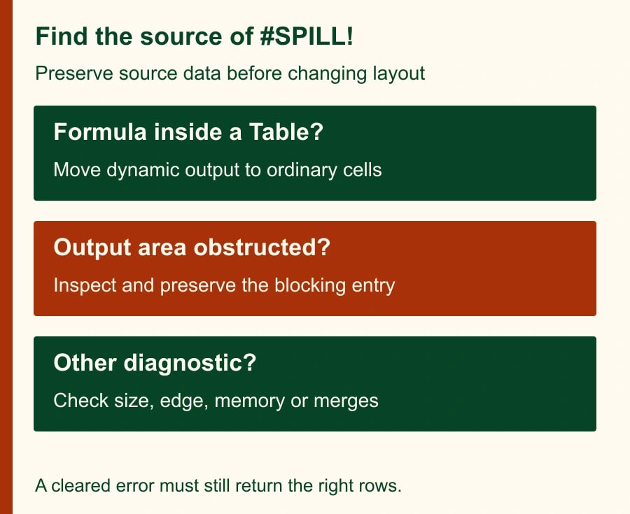
Before moving an obstruction, identify its owner and purpose. A small note under a report may be an analyst’s only record of a disputed order. A cell that appears empty deserves inspection in the formula bar before you clear it. The correct recovery can be moving the report, relocating the note with its context or reserving a different output sheet. It is not necessarily deleting the obstruction.
Keep the source as a Table
An Excel Table is a named, structured set of records. For this workflow, it is the controlled input, while the spill area is a view of selected records. Keeping the roles separate makes the workbook easier to maintain: staff update the source, and the formula determines which rows appear in the action list.
Put the result on a dedicated worksheet if the existing report is crowded. Place a short instruction above it: edit records in the source Table; do not type into the generated result area. Keep a generous clear area beneath and beside the formula, sized for the largest plausible output rather than today’s small sample. A list that has room for three results today may need room for thirty tomorrow.
If a colleague wants comments beside each generated row, agree on a durable record key first. Store the comment against that key in a separate controlled list or the appropriate source system. Otherwise a result can move while an adjacent manually typed comment stays in the old row. The workbook can look neat and still attach the wrong explanation to a customer.
Do not convert the source Table to a plain range simply because a troubleshooting page lists that as an option. It can be appropriate in a deliberately redesigned workbook, but it changes a useful structure. For a separate action list, moving the formula is usually the smaller change. Review dependent formulas and refresh processes before changing the source’s structure.
Build the five-row example
Create a test Table named Orders with these four columns in this order: Order ID, Customer, Amount, Status. Use numeric values in Amount. The example currency is dollars, but the formula does not perform currency conversion. Enter the following invented records; the names are labels for the exercise, not customer results.
- O101, Alder, 240, Ready.
- O102, Birch, 180, Hold.
- O103, Cedar, 360, Ready.
- O104, Dogwood, 120, Ready.
- O105, Elm, 500, Hold.
On a separate ordinary worksheet called Ready List, type Order ID, Customer and Amount in A1:C1. Leave the area below clear. Enter this formula in A2: =FILTER(Orders[[Order ID]:[Amount]],Orders[Status]="Ready","No ready orders")
The first argument returns the three adjacent columns from Order ID through Amount. The second checks each Status for Ready. The final argument supplies a readable message when nothing matches. Microsoft’s FILTER documentation describes these arguments and notes that an omitted empty-result argument can produce #CALC!. That is a different problem from a blocked spill.
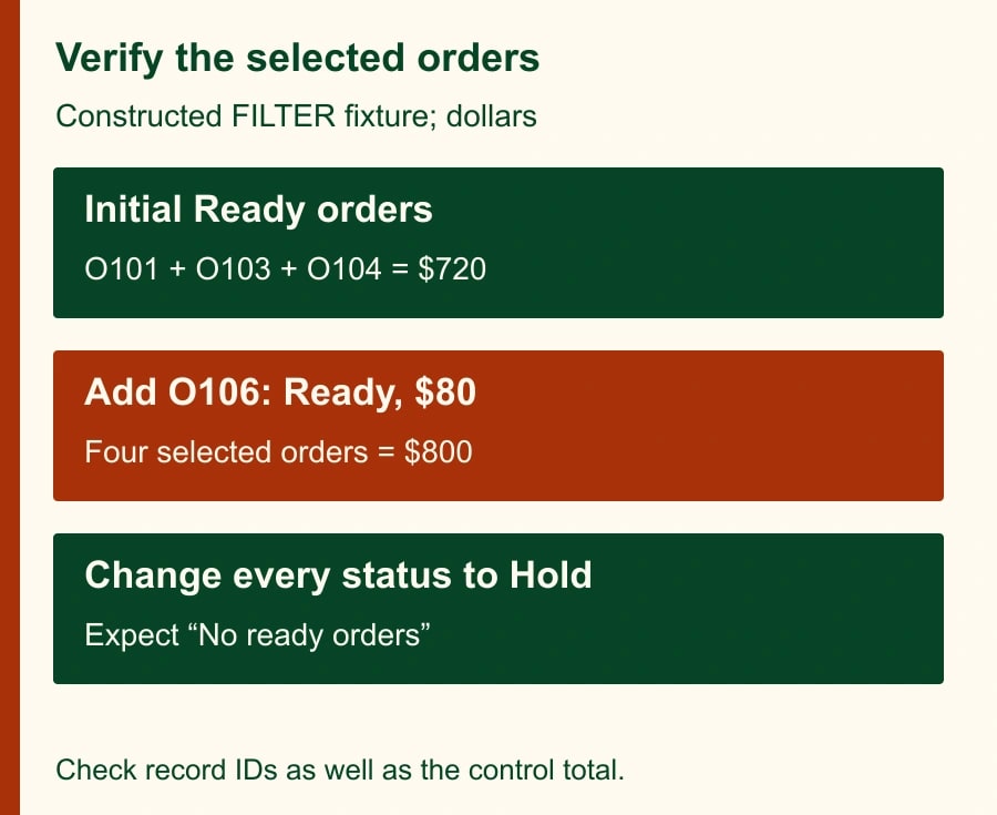
The expected output is O101/Alder/240, O103/Cedar/360 and O104/Dogwood/120, occupying A2:C4. The selected amount is 240 + 360 + 120 = 720. The full source amount is 1,400. The two held orders account for the remaining 680. These totals are controls for this fixture; the output is not an invoice approval or permission to release an order.
Read the actual IDs as well as the sum. Three incorrect rows can coincidentally total the same amount as three correct rows. For a live queue, keep the business owner’s selection rule alongside the formula so the analyst can explain why each row belongs. Status labels alone may be insufficient if readiness also depends on payment, stock or an approval stored elsewhere.
Prove that the result can grow and become empty
Add O106, Fir, 80, Ready to the source Table in the test copy. The expected action list now has four rows and totals 800. The output should extend to row 5. This test is more useful than repeatedly checking the original three-row result because it tests the space you have reserved and the source reference’s ability to include new records.
Next, place a clearly labeled temporary test entry where a future output cell would be, using only the disposable test copy. Add enough matching records to reach it. Confirm that the obstruction is visible through the error diagnosis, then remove only your temporary test entry. Do not rehearse this by inserting junk into a live order queue or deleting a colleague’s notes.
For the empty test, temporarily change all Ready statuses in the copy to Hold. The expected result is the message No ready orders. Treat that message as a state to handle, not as a record with an amount of zero. A downstream export that expects three numeric columns needs its own empty-state handling; a human-readable message is not automatically suitable input for another system.
Restore the fixture and verify the original IDs and 720 total again. This final return check catches accidental changes introduced during testing. Keep the test copy or a short record of the expected results so someone else can repeat the exercise after a workbook redesign. Do not substitute a screenshot of one successful result for the growth and empty tests.
Avoid fixes that change the question
Adding @, narrowing a reference to one row or replacing an array with a single-cell lookup can remove a multirow result. Those choices can be correct for a one-value-per-row calculation, but they do not preserve an action list whose job is to return every matching record. Microsoft’s error guide distinguishes single-value approaches from dynamic output. Review the intended answer before accepting a formula suggested by an assistant or a forum.
Use a simple review prompt if an AI assistant is helping: “Explain the intended output shape of this formula. Identify whether your proposed change returns all matching records or one value. Do not change the selection rule. Show the expected IDs for my synthetic fixture and list assumptions.” Give it the constructed rows rather than confidential customer data unless your organization has approved that use.
Then verify the proposal yourself in a workbook copy. A fluent explanation is not evidence that the formula preserves a business control. If the suggestion silently drops the status condition or changes a many-row list to a single result, reject it even if #SPILL! disappears. The absence of an error is a technical symptom, not a definition of correctness.
If the formula depends on another workbook, check that dependency separately. Microsoft notes limited support for dynamic arrays between workbooks, with both needing to be open for supported operation. A closed-source refresh can produce #REF!. Moving the output area will not fix that dependency. Decide whether the workflow needs a more reliable imported dataset before using it for unattended reporting.
A repair record the next analyst can use
- Workbook copy and owner: identify where the diagnosis was performed and who approved the live change.
- Business rule: state exactly which records belong, including exclusions and missing-status handling.
- Source: record Table name, column order, record key and amount type.
- Formula anchor: record the top-left output cell and whether it is outside a Table.
- Error cause: capture Excel’s diagnostic and the specific obstruction or structural issue.
- Preservation: record what was moved, where it went and who confirmed that nothing important was deleted.
- Tests: check expected IDs, control total, growth, empty result and restoration of the original fixture.
- Handoff: identify where manual notes belong and who investigates future errors.
Keep the repair small enough to explain. If you have changed source structure, formula logic, column order and downstream export handling at once, it will be difficult to identify the cause of a new discrepancy. Separate the layout repair from any planned redesign and validate each against the same business rule.
Know when the workbook needs a different design
Stop the local fix if the output must support many people editing individual results, if record identity is unreliable or if the queue drives irreversible actions without a human check. A formula view can help someone review work; it does not provide a full assignment history or transactional workflow. Escalate those requirements to the system owner rather than adding more fragile columns around the spill area.
Measure success by correct records and a repeatable refresh, then track time spent repairing the queue. For a constructed example, reducing four weekly ten-minute repairs to one five-minute check releases thirty-five minutes per week. That is capacity, not cash savings, and it excludes the one-time redesign effort. Use observed repair logs before claiming that outcome for your team.
Start with a copied workbook and the five-row fixture. When the source remains intact and the output passes the growth and empty checks, apply the smallest approved layout change. If the source itself contains invalid statuses, use the guide to Excel data validation that fails after pasting. If duplicate records are inflating the control total, investigate Power Query merges that multiply rows before blaming the spill area.
Weekly Newsletter
AI Adoption Weekly
New research, field guides, training studies, and tool decisions for operators.
No spam. Unsubscribe anytime.
Related Comparisons
Calculator
AI seat cost calculator
List price × headcount. You enter the hours and the operating assumptions.