Excel filtered totals: When to use SUBTOTAL 9 or 109

Use SUBTOTAL(9,…) when a filtered Excel list should include rows a colleague hid by hand. Use SUBTOTAL(109,…) when the subtotal should reflect only the rows still visible. Both ignore rows removed by a filter. For a number that must stay fixed when someone changes the view, neither is the right definition: calculate from explicit business criteria and label that total separately.

The distinction matters when a sales manager sends a pipeline estimate to finance. A row hidden to keep a meeting screen tidy is still a real order. A row removed by a region filter may be deliberately outside the manager’s remit. Deciding which orders count is the manager’s job. A spreadsheet formula can follow the decision, but cannot make it.

Find out what the number above the list promises

Read the cell label as though you were the person signing the forecast. “Total” could mean all open orders, all orders in the selected region, or only the orders under discussion today. Those can be three different amounts in the same workbook. Write a sentence precise enough that a colleague could reproduce it without seeing your screen. If you cannot do that, postpone the formula change and ask the report owner to name the population.

There are two good reasons to want a moving total. Someone exploring a long pipeline wants the number to change as they filter. Someone walking through a small set of disputed orders may want it to change again when a reviewed row is hidden. A signed monthly forecast has a different purpose. A recipient reopening it with different filters should not be able to change what the team committed to simply by changing the view.

Microsoft’s SUBTOTAL reference explains the numbered choices: 9 and 109 both sum values, and differ in their treatment of manually hidden rows. They work down a vertical list. Hiding a column in a horizontal range does not give the corresponding result. The method below requires Excel, a copy of the workbook, a vertical numeric amount column and a known handful of orders. It does not require an add-in, an AI subscription or a new dashboard.

Build a five-order sheet before touching the real forecast

Constructed example: put Order, Region and Amount in A1, B1 and C1. Enter A, East, 120 on row 2; B, East, 80 on row 3; C, West, 200 on row 4; D, East, 50 on row 5; and E, West, 150 on row 6. Use actual numbers in the amount cells. Put the check formulas outside the rows you plan to hide. For example, enter =SUM(C2:C6), =SUBTOTAL(9,C2:C6) and =SUBTOTAL(109,C2:C6) in F2, G2 and H2. Leave row 2 visible throughout this exercise.

With no filter and no hidden rows, all three results are 600. That agreement proves little by itself. A formula that follows visibility and one that ignores it will always agree when everything is visible. The diagnostic part is deliberately changing one property at a time and writing down which result should change before you touch the sheet.

Turn on a filter on A1:C6 and select East in Region. Rows for orders C and E disappear. The ordinary sum stays 600. Both subtotals read 250, from 120 + 80 + 50. Now right-click the row header for B (row 3) and hide that row manually. The ordinary sum is still 600. SUBTOTAL with 9 remains 250 because B still qualifies as East. SUBTOTAL with 109 falls by 80 to 170. The 80 has not vanished from the pipeline; you have changed what one reporting cell promises to count.

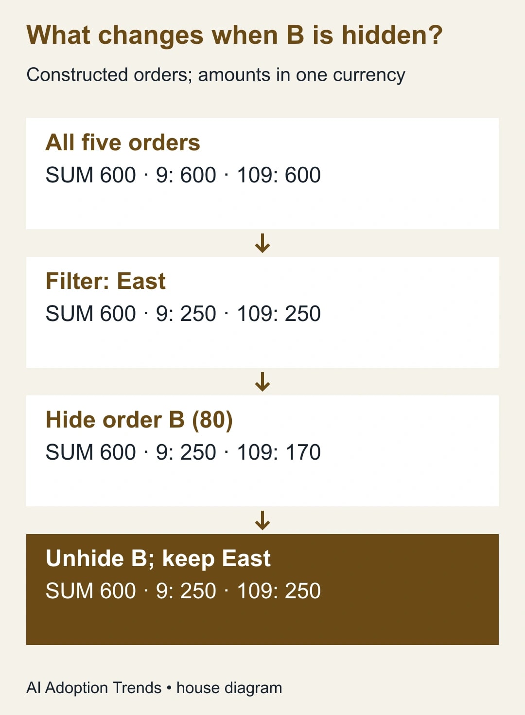
Unhide B while keeping East selected. The two subtotals agree again at 250. Clear the filter after that, then confirm all three return to 600. Doing these repairs in the opposite order can make it hard to tell whether a manually hidden row remains hidden on your particular sheet. Use the known order identifiers as the check. Five rows back on screen is stronger evidence than a filter icon that looks inactive.

When a view is useful and when it becomes a liability

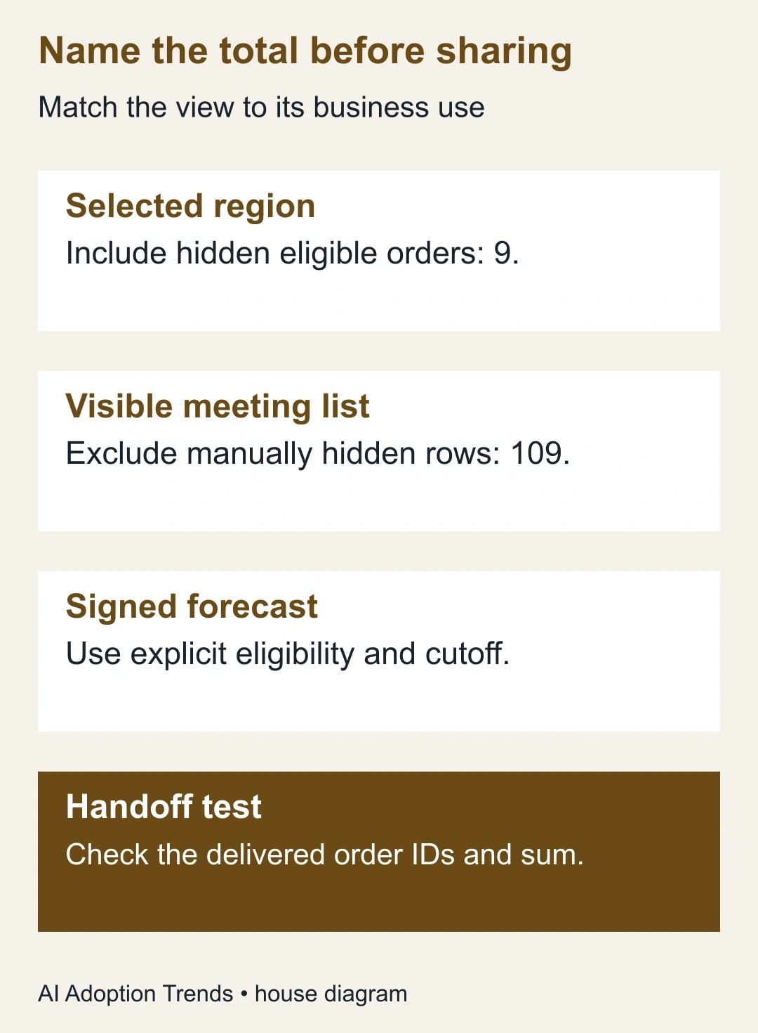
Suppose the manager hides B because a colleague is talking about it on another call. For an East region forecast, it still belongs. Label the 9 result “Selected regions, including manually hidden orders.” For the current meeting, a 109 result labeled “Visible orders on this screen” is a fair account of what participants can see. Both are accurate at once. Avoid a generic label that makes the second number look like a revised regional commitment.

Now suppose B is a duplicate that should never count. Hiding it by hand is a poor repair: the apparent fix depends on the formula and is easy to undo. Add a reviewed exclusion field with the actual reason, or correct the duplicate in the source after the owner approves it. Rebuild the committed forecast using that rule. A future import can reintroduce rows without their display state, while an explicit order identifier and exclusion reason can be checked again.

For a handoff, write a separate figure such as “approved East orders at 5 p.m. Friday.” Record the cutoff, source version and eligibility conditions. In the five-row example, if all East amounts are eligible, =SUMIF(B2:B6,"East",C2:C6) gives 250 even when B is manually hidden. In a real forecast you may also need approval status, close date and currency; use a maintained set of criteria and validate each one. Geography alone does not make an order approved.

Diagnose an unexpected total in the right order

First inspect the actual formula and its reference. A subtotal can be correct on C2:C6 while the new order on row 7 sits completely outside it. Put a known new order in a working copy and verify the range expands or is deliberately maintained. If the total looks right merely because a missing row offsets a duplicated row, comparing amounts will not reveal the mistake. Compare the identifiers in the expected group too.

Next, check the amount cells that look numeric. A currency symbol rendered by formatting is different from a text string pasted from another system. Try a known numeric row and a suspected text row separately in the working copy. Do not convert a whole source column in place before checking currency, separators, blanks and any legitimate text markers. “Unknown” and zero are different promises to finance.

Then inspect summary rows embedded among orders. Microsoft documents that SUBTOTAL ignores nested SUBTOTAL results in its range to avoid counting those subtotals again. A manually typed summary, however, is just another number. So is a summary returned by a different type of formula unless you explicitly keep it out of the detail range. A row labeled “East total” in column A is not an instruction to Excel. Keep a clean order-only range and put summary calculations outside it.

Check what the recipient is actually opening. A pasted value in a slide cannot respond to a filter. A new download might open with all rows shown. An automated import could read the underlying order records rather than the subset visible on someone's screen. If the job is a fixed export of eligible orders, produce the actual subset explicitly, attach its count and amount and verify the delivered file. A correct number displayed in the source workbook is only one part of that handoff.

Run the handoff once as the person who gets the report

Make a duplicate of the five-order example for a colleague. Supply the field definitions and the two formula labels, but leave the row filters in the state used during the meeting. Ask them to recover the East total for the forecast and the amount the meeting participants saw. They should be able to explain the difference of 80 by naming B. If the only way to identify it is to remember what the presenter hid, the worksheet needs a visible inclusion or review-status field.

Now change the exercise. Tell the colleague that B has been excluded from the forecast under a documented sales rule but still needs to appear on the meeting list for discussion. A single filter on visible rows cannot express both requests at once. The report needs two definitions: what people should see and what finance should count. Keep the row visible, record the exclusion reason and count only records eligible for the forecast in the committed figure. Hiding evidence of the exception makes the meeting easier to read but the decision harder to explain later.

A useful request to a spreadsheet assistant is: “My amount is in column C. I filter rows by region, and I also hide some rows manually during a call. Give me separate formulas for the filtered regional amount and the currently visible amount. Predict both results after I hide an eligible order for 80. Explain which result finance should use if the forecast must never depend on the current view.” Give the assistant the five fictional rows rather than the live deal list. Reject an answer that predicts the same change in both subtotals or proposes a view-dependent formula for a fixed forecast.

If you're replacing an existing formula, trace its consumers before renaming or moving the cell. A linked slide, a copied meeting note and an automated export may each rely on a different meaning of “total.” Give the new visible figure its own location and compare deliveries for one reporting cycle before redirecting the old reference. The success measure is whether each recipient gets the intended rows and named amount, including on days when someone has filtered the sheet differently. A correct live screen alone cannot answer that question.

Acceptance note for the workbook owner

• What the total means: fixed business rule, filtered group including manually hidden rows, or currently visible rows.
• What it includes: source table, amount field, unit or currency, exclusions, cutoff and responsible person.
• Five-order check: all rows 600; East only 250; East with B hidden 250 under 9 and 170 under 109; all rows restored 600.
• New-order check: append one known order in a copy, confirm where it counts, then remove it or discard the copy.
• Distribution check: confirm the cell label, saved filter state, row count and amount in the file the recipient actually uses.

For an analyst, the cost of this repair is the time to map which downstream reports use the cell and retest those links. A workbook used only during a meeting can be changed quickly. A workbook feeding commissions or a board pack deserves its own version and a second reader. Keep the original until the consuming report has passed the same order-level check. If two teams need different meanings, give them separately named cells rather than switching a shared cell back and forth.

Choose one live total today and ask the recipient what should happen when an eligible row is hidden by hand. Their answer selects the formula or exposes the need for a fixed business rule. If the result later moves between spreadsheet products, the pivot table handoff checks for Sheets and Excel offer a separate test for what survives the transfer.